Here is the link to the Practicals Page for Lesson 2. I will add new assignments every day or so to help you create a single page document. For now you can find the raw .Rmd file on GitHub. The link is in the title of the Practicals Page.
R Markdown is a versatile framework for creating a range of high-quality documents including HTML, PDF, presentations, books, websites, and more. Markdown allows documents to be simple and portable while R integration gives you the benefit of creating dynamic documents that contain your results (e.g., tables, graphics, and inline values). Results can be computed and rendered dynamically from R code and are more likely to be reproducible.
Learning Objectives
In this section of the course, you will create a single page R Markdown document and then turn that document into an HTML page. The lesson itself (this document) is designed to lay down the conceptual and mechanical framework you need to get started. Your job is to understand this material because it is the basis for everything that comes after. I included many links to additional resources, so if a concept is unclear, spend some time going through the links I provided. If you do not understand something, please ask. Chance are pretty good that you are not alone.
After you go through this lesson (and understand the concepts :), you will start working on your single page document. In parallel, I will release my own single page document with assignments and challenges. That way we can work on our documents together and I can demonstrate how to accomplish certain tasks. The entire session is designed to last two weeks.
Self-Paced Tutorials
You should also be working on the self-paced tutorials. The command line interface tutorials are included to get you accustomed to the command line environment. In addition to simply being an invaluable skill, you will use the command line when we work on git and GitHub integration. You need to have some basic navigational skills including how to list files and hidden files as well as how to edit, rename, move, delete, and create, files.
Assignment
Over the next two weeks, you should complete the following tutorials: A Command Line Crash Course and Basics and Navigation. I listed two videos on the Tutorials Page that are recommended viewing.
I included a tutorial for HTML & CSS because at some point you will run into a situation that requires a basic knowledge of these languages. Please complete the following lessons over the next two weeks from Interneting is Hard: Introduction and Basic Web Pages.
Lesson Overview
-
This lesson will cover the following:
- how an HTML page is generated from an R Markdown document;
- the structure of an R Markdown document and
- its three main components—the YAML header, Markdown text, & R code chunks; and finally
- how to run Inline R Code.
Rendering a Document
Before we start, I want to give you a little overview of how an HTML document is created from Markdown-formatted text and R code. The process is called rendering—where the input file(s) are transformed to a specified output format, like HTML.
When you render an R Markdown document you use a program called knitr. Knitr executes all the R code, knits the results together with the Markdown text, and creates a new Markdown document. The new Markdown document is then processed by PanDoc, which converts the Markdown syntax into HTML and CSS code. PanDoc is like a swiss-army knife for Markdown—it can covert many types of Markdown documents into a variety of other formats. Don’t worry, all of these steps happen behind the scenes. As long as you have a properly formatted R Markdown document, these tools will take care of the rest.

Familiarize yourself with knitr and PanDoc. Even though they are doing the work for you, understanding what each does and how they do it will help you troubleshoot problems. Links are provided in the image above.
Structure of an R Markdown Document
A basic, single page, R Markdown document is created from just three elements: the YAML header, Markdown-formatted text, and R code chunks. Technically, you do not even need R code; many of the pages on this site have no R code at all. But for our purposes, we will incorporate R code as a necessary ingredient so that you can experience the potential of R Markdown. Even if you don’t know much R, I want you to use R code in your document. Later in the lesson, I briefly introduce built-in datasets that you can use, and I am happy to provide you with any additional advice you may need. Many of your classmates are expert R coders, so please ask for help on the #data-curation Slack channel.
Additional customization of an R Markdown document can be achieved with user-defined CSS and/or HTML code, both of which will be the subject of a future lesson. For this lesson, we focus on the three core elements—YAML, Markdown, and R code chunks.
The YAML header
At the top of an R Markdown document you must include YAML metadata as the header. YAML (a meaningless acronym that stands for YAML Ain’t Markup Language) is human readable—meaning that the syntax is easy to read and write. YAML metadata is used to configure the settings and parameters of a document or program. Since it is used by PanDoc, the YAML metadata technically comes into play during the final step of the pipeline. But since it is usually at the top of a document, I will cover YAML first.
We control how PanDoc configures our rendered document by populating the metadata with different options. For examples, we can specify the type of document we want PanDoc to construct—HTML, PDF, Word, etc. We can also include a table of contents (toc) or specify a theme. Themes allow you to set the look of the document—the font style, coloring, etc. Each theme comes prepackage with its own CSS and HTML code that PanDoc applies to the final document. We will cover themes more extensively during the tutorial part of the lesson. I’ve listed some of the theme options in the YAML section of the Resources page.
All YAML header options are tied to built in functions. What this means is that we need to know what the YAML options are and what each one does. A YAML option consists of a pair of values—an argument + a property. For example, if we want to add a date to our document, we include the date argument and then pass a property to that argument. However, something like agouti is not a YAML argument and nothing will happen if you try to use it. If you want to control a component that is not a built-in function, you must include additional instructions like custom CSS and HTML code. This is not too difficult, but it is a topic for another day. A side note—on the Web, you may see argument referred to as a key and property referred to as a value. I am not aware of a strict naming convention, but I will do my best to be consistent and use the argument/property pair.
For a single page document like the one you will create in this lesson, the YAML metadata must be enclosed in delimiters. We will use delimiters a lot, so make sure you understand the concept. For YAML headers, we use three consecutive dashes (---) without spaces. The delimiters must be on their own lines and you must add the YAML metadata between the two delimiters. Like so…
---
Some YAML metadata
---
YAML options
The structure of a YAML option is
argument: propertypair where argument is a built-in function and property is the information you pass to the argument.
There are many arguments you can include in your YAML header, some of which are general and others that only apply to specific document types.
Further Reading
Please spend some time looking at The YAML Fieldguide, in particular the sections called Basic YAML and R Markdown Websites. Most of the YAML arguments we can use for our project are listed in these two sections. Each entry contains the argument name, a description of what it does and how to use it, and a link to a help page. The help pages contain additional details and examples.
Assignment
Open R Studio and go to File > New File > R Markdown. A window like this should pop up where you can fill in the details. It is not important what you put here since you can change it at any time. What is important is that Document and HTML are both selected. Hit Ok.
New R Markdown document window.
Once you hit Ok, a new R Markdown document is created and opened in the Environment window of RStudio. Let’s take a look, but for now just focus on the top of the page.
---
title: "DC Lesson 2 Single Page Document"
author: "Jarrod"
date: "4/7/2020"
output: html_document
---
This is the YAML header of the R Markdown document you just created. As you can see, the format is simple. R Markdown took the information I provided in the set-up window and populated the header with some basic YAML metadata. Each line has a YAML argument followed by a colon : and then a property. Any information you put in the YAML header must be in this form; however, you can include comments by using a hashtag (#) at the beginning of a line.
Notice that some of the properties, like the name of the author or the title of the document, are in quotes, while the property for the output is not in quotes. Why is this the case? Good question. For the sake of explanation, let me categorize properties into two classes—variables and operators.
- Variables: A variable can be any string you want (a string is just a sequence of characters). For example, I could set the property of the
authorargument like thisauthor:"Iamtheauthorofthispaperhearmeroar". For arguments likeauthor,title, etc., PanDoc doesn’t care what property you set. It knows these arguments can take pretty much any string you pass it. - Operators: Think of an operator like a choice. The
outputargument here is set tooutput: html_document. The propertyhtml_documentis one of the choices you have for this argument. If you enter a property that is not in the list of choices, you will get an error, and your document will not render. Likeoutput: cold_beermay work in some situations but not in our YAML header.
The convention is that variable properties are enclosed in quotes and operator properties are not. The argument itself is never quoted.
Now that I told you all of this, I also need to tell you that most of the time, quotes for variable properties are optional. However, putting variable properties in quotes allows you to include special or reserved characters in your string. For example, let’s say you want to set the author property to your Twitter handle, @cool_coder (I think this handle is available :). The @ sign at the beginning of a string has a special meaning for PanDoc. If you do not put this string in quotes, you will get an error and your document will not render. By writing the option like this—author: "@cool_coder"—with the property in quotes, you can use the @ sign and everything works fine. There is a lot of confusion on the Web about when to include quotes and when not to. My best practice advice is to always use quotes with variable properties. Symfony has a pretty good breakdown of quote usage in variable strings.
Assignment
Go ahead and customize your YAML header with a name and title. Now hit the knit button just above the text editor window. There is a little dropdown menu that lets you select the type of document to produce, but since you have already specified output: html_document, you can just hit the button. RStudio will prompt you to save the document. Do not add a file extension. RStudio just needs a root name.
File naming
A note on file naming best practices. You can save yourself a lot of trouble by following a few simple rules when naming files.
Make sure your files are Machine readable and Human readable.
- Never use special characters in your file name (e.g.,
* # : \ / < > | " ? [ ] ; = + & £ $, and so on). Letters and numbers only. A lot of software will reject files that contain these symbols. Periods.should only be used for a file extension, likedocument.html. - Do not use spaces. Separate words using a dash (
-) or an underscore (_). This is an exception to rule #1. - The file name should be meaningful. This is important when dealing with a lot of files, like for a website. So add relevant details.
- But do not make the names super long either. Long file names mean long URLs, which can increase the likelihood of errors.
- Capital letters are ok, but they can make autofill a pain. This is a matter of personal preference.
Once you hit save, RStudio will render the document following the process I described above. Do you see any errors in the Console window? No? Good. What about a new .html document in the working directory? Yes? Also good. Double-click that file and it should open in your default browser. Does it look something like this?
If so, congratulations. You just created your first web document. I admit, it is a little boring at the moment, but this is all it takes to make a basic page. There is one more aspect of YAML headers that I want to touch on before moving on.
Nested YAML options
I have discussed the structure and components of YAML headers, specifically delimiters for demarcating YAML metadata, hashtags # for including comments, and argument: property for setting options. To complete our initial explanation of a YAML header, we need to talk about nested options.
Think about an unordered list for a minute.
- Item A
- Item B
- Item C
The list has three elements and each line begins with a new element. Let’s also take a look at the Markdown code for the list.
* Item A
* Item B
* Item C
The structure of this list is similar to the YAML header in our document.
title: "DC Lesson 2 Single Page Document"
author: "Jarrod"
date: "4/7/2020"
output: html_document
Ok, now let’s construct a nested list. A nested list is a composed of parent elements that have their own list of elements called children—lists within a list. In this example, A and B are parent elements because each has their own list. C on the other hand, has no child element.
-
Parent A
- Child A1
- Child A2
-
Parent B
- Child B1
- Item C
If we compare the Markdown code of the nested list to the normal list, we see an important difference. The child elements of the nested list are all indented. We need indentation to construct a nested list and we get indented code by using spaces at the beginning of child lines.
* Parent A
   + Child A1
   + Child A2
* Parent B
   + Child B1
* Item C
If we want more control over the structure of our document, we need to incorporate nested elements in the YAML header. The first thing you need to know about nested elements is that YAML doesn’t allow tabs for indentation, meaning you must use one or more spaces for indentation.
Ok, now go back to the YAML header of our document and add the argument theme and the property journal so we can specify the look of the final product. Remember, the format is argument: property
title: "DC Lesson 2: Single Page Document"
author: "@cool_coder"
date: "4/7/2020"
output: html_document
theme: journal
I save the file, run knit, and look at the output. Hum. Nothing changed. This is because theme is not a general PanDoc argument like title, author, and date. The theme argument is specific to the property of the output argument. To see what I mean, please find theme in the PanDoc options section (Page 5) of the R Markdown Reference Guide. What you will see is that theme can only be set for two document types (HTML & Beamer).
Truncated view of the PanDoc options section from the R Markdown Reference Guide.
If you look more broadly at this section you should notice that most options can only be used with specific document types. Please note, you will often see option and argument used interchangeably. This is annoying. Again, I will use the term option to refer to an argument plus it’s property.
Ok, in order to use theme, we first need to make sure we are using the property for output. Check. Next, we need to make theme as a nested element of the output property html_document. In doing so, html_document becomes both the property of output and the argument of theme. Since we cannot have two arguments on the same line, we need to set html_document as a nested element of the output.
title: "DC Lesson 2: Single Page Document"
author: "@cool_coder"
date: "4/7/2020"
output:
  html_document:
    theme: journal
I know, this is super confusing. I spent hours just trying to explain it to myself. Think of it this way—start from the bottom of the YAML metadata above and work your way up.
journalis a property of the argumenttheme.themeis a property of the argumenthtml_document.html_documentis a property of the argumentoutput.outputis the parent argument.
In essence, a nested list of options. Anytime we want to add a new option, we need to know what it is, what it does, and whether it is a parent or child. Please make sure you understand these concepts before moving on. A properly formatted YAML header is a key step in creating a document. We will cover YAML headers in greater detail during the exercises. For now, I want to cover the remaining components of the document.
Markdown Formatted Text
Now it is time to add some content. Any document you create needs some text or else it is just a bunch of code and not very fun to read. But remember, in R Markdown the text is formatted using Markdown syntax. I already covered the basics of Markdown so I will not spend any more time on it here. Markdown syntax is pretty straightforward. Use the reference guides on the Resources Page to get started. Still feeling a little lost? Try this brief but excellent Interactive Markdown Tutorial. Each lesson contains a brief explanation of Markdown syntax. Hit the Try it button to test your skills and see what your solution looks like when it is rendered. There is also an option to see the HTML equivalent of the Markdown text. This is a nice tutorial.
Assignment
In your new R Markdown document, add some Markdown-formatted content. If you already have some text, feel free to add it. If not, use a Lorem ipsum generator to make a bunch of plain text that you can add to your page. Your assignment is to use Markdown syntax to format the document. Add headers, links, make some text bold or italic, etc. Structure your document like you would a real page or project. Your goal here is to get comfortable with Markdown and the best way to do that is to practice.
To see any changes you make, you must save the document and run
knitagain. Make sure you have no errors and refresh your browser.
R Code Chunks
If you have used R before, you know there are a couple of ways to run code. You can run commands interactively in the console or use batch processing to run a script. You may choose to send the results to a file (like a figure or table) or simply print the results to the screen. If you have never used R, I suggest investing some time learning this amazing tool. There are hundreds of tutorials and courses online, many of which are free. For example, Bill Petti offers a nice Crash Course in R that covers some of the basics. You do not need to be an R expert to go through this course, but some understanding of R is very helpful. If you are an R expert, please consider posting resources to the #data-curation channel, and I will add them to the Resources Page.
Running code in an R Markdown document is very similar in principle to how its run in an R console. Remember, when you render an R Markdown document, knitr first executes all of the R code. But knitr needs to know which text in the document is R code. To differentiate R code from normal text we use code chunks. I will show you what I mean.
When we open a new R Markdown document, the software is kind enough to include a few examples of Markdown text and R code to help us get started. R comes with several built-in datasets (thanks to the datasets package), which are generally used as demo data for playing with R functions. In your R or RStudio console, simply type data() to see a list of the built-in datasets. We will use these datasets in an upcoming post on Solving Problems (Part 2) when we discuss Minimal, Reproducible Examples. You can also use the built-in datasets for this exercise, so please study up.
Anyway, if you go back to the .Rmd file that you generated and scroll down a little, you will find an example of R code. R Markdown is using the cars dataset from the datasets package as the example.
```{r cars}
summary(cars)
```
This is called a code chunk. There is another code chunk at the top of the .Rmd page (just below the YAML header) but we will come back to this later because it is a little special.
I covered the general concept of code chunks in Lesson 0, but this piece of the puzzle is important, so I want to discuss it in more detail here. Like our YAML header, an R code chuck is distinguished from the rest of the text with delimiters, in this case three consecutive back ticks without spaces (```). Think of a code chunk like a mini R environment. Knitr essentially pulls the code out of the chunk, runs the code in R, and then puts the results in a new document as Markdown-formatted text. Code chunks can also have options, which are enclosed in curly brackets. We will get back to chunk options in a minute.
Running R code
Open the .html file generated when you rendered (or knitted) the R Markdown document and scroll to the part that corresponds to the summary(cars) section. This R command simply calls the summary function against the data frame cars.
The image on the left is a screenshot from that section of the HTML document. The first thing you should notice is that there are no delimiters or any information about the chunk, just the command summary(cars). I will explain this in a second. Below that is a box with some data. We certainly didn’t code this data into our R Markdown document—these data are the results of running the command. We asked for a summary of cars and that’s what we got.
Left, code chunk output from the HTML document. Right, output from the R console.
On the right is a screenshot of my R console. I just copied the command and ran it in R. I hope you can see that aside for some formatting differences, these results are identical. This is because knitr is running the code in R and encoding the results in Markdown, itself translated to HTML by PanDoc. Ninety-five percent of the time, all you need to do is paste your R code into a code chunk and it will be processed like this. Of course, nothing is absolute, and we will encounter some exceptions.
Where are the chunk details?
You cannot see the chunk details because they are hidden. Chunk details are instructions for knitr on how chunks should be rendered. This information is not important for reproducibility or transparency, so it is hidden. Anytime you do see code chunk information on a page, it is because that chunk is intentionally being rendered verbatim. Normally we do this for demonstration purposes only. From now on, I will only show code chunk information as a learning tool. Otherwise it will be hidden, and you will have to dig around on GitHub to find it :)
Chunk structure & options
Great. Let’s review the structure of a code chunk. Below is an annotated screenshot of a piece of code I wrote to define a simple color palette. If you haven’t worked much with colors, the strings preceded by hash tags (#) are called hex codes. Hex codes are great for encoding color in many languages including R.
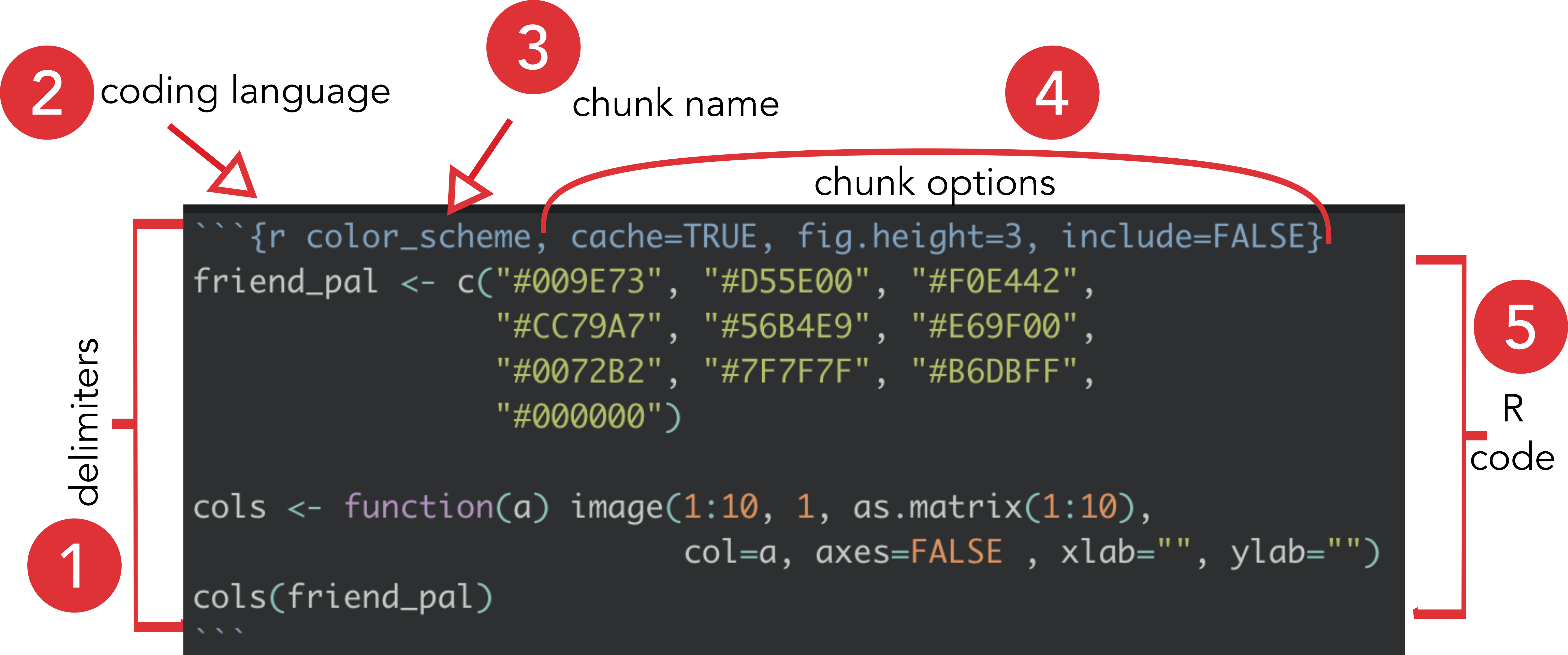
Example code chunk illustrating the formatting & different components.
The format of the code chunk is as follows:
- Delimiters: Often called a code fence, delimiters partition your code from the rest of the text. For R Markdown we must use three back ticks.
If we stopped there and didn’t not add any more information, the final document would only contain the text between the delimiters, formatted like this:
friend_pal <- c("#009E73", "#D55E00", "#F0E442",
                "#CC79A7", "#56B4E9", "#E69F00",
                "#0072B2", "#7F7F7F", "#B6DBFF",
                "#000000")

cols <- function(a) image(1:10, 1, as.matrix(1:10),
                          col=a, axes=FALSE , xlab="", ylab="")
cols(friend_pal)
Without any other information, knitr recognizes the delimiters and knows its code. But since no other information was provided, knitr does not run the command or generate any results. It simply takes the chunk and turns into Markdown-formatted text. This can be useful if you want to call out a block of code without running anything. But if you want knitr to actually do something with this command, you need to provide more information.
- Coding Language: To run code, the minimum information you need to include is the name of a language enclosed in curly brackets (
{ }).
R Markdown supports many languages like Python, BASH, and of course R. For example, I can call BASH and run a simple command like I would from the CLI. I can use the ls command to list all the files in a directory and add the l flag to get a long listing for every file, a to include any hidden files, and h to return file sizes in human readable format. Please pay attention to the structure of the chunk.
```{bash}
ls -lah
```
## total 456
## drwxr-xr-x 20 rad staff 640B May 18 08:15 .
## drwxr-xr-x 6 rad staff 192B Mar 31 11:38 ..
## -rw-r--r--@ 1 rad staff 6.0K Apr 14 17:46 .DS_Store
## -rw-r--r-- 1 rad staff 0B Apr 5 10:34 .Rhistory
## -rw-r--r--@ 1 rad staff 14K Apr 6 20:51 help.md
## -rw-r--r--@ 1 rad staff 15K Apr 11 06:02 lesson-0.Rmd
## -rw-r--r-- 1 rad staff 16K May 18 08:15 lesson-0.html
## drwxr-xr-x 4 rad staff 128B Mar 30 05:10 lesson-0_cache
## drwxr-xr-x 4 rad staff 128B Mar 30 05:10 lesson-0_files
## -rw-r--r--@ 1 rad staff 27K Apr 20 07:24 lesson-1.Rmd
## -rw-r--r--@ 1 rad staff 29K May 18 08:15 lesson-1.html
## drwxr-xr-x 3 rad staff 96B Mar 30 08:47 lesson-1_files
## -rw-r--r--@ 1 rad staff 36K May 18 07:54 lesson-2.Rmd
## -rw-r--r--@ 1 rad staff 41K May 18 07:54 lesson-2.html
## drwxr-xr-x 3 rad staff 96B Apr 8 20:57 lesson-2_files
## -rw-r--r--@ 1 rad staff 2.4K May 18 08:13 practicals.Rmd
## -rw-r--r-- 1 rad staff 2.5K May 18 08:13 practicals.html
## -rw-r--r--@ 1 rad staff 4.2K Apr 1 08:59 rationale.md
## -rw-r--r--@ 1 rad staff 2.6K Apr 15 11:15 reproducibility.Rmd
## -rw-r--r-- 1 rad staff 3.0K May 18 07:54 reproducibility.htmlBy specifying a language, knitr was able to interpret the code and run the commands. And as you can see, I got a printout of the results right in the final document. Of course, in our case, we will mainly use the r language option. But you may want to explore the functionality of other languages in your own work.
- Chunk name: The name must be unique, it needs to come right after the language variable, and it must be separated by a space.
Adding a chuck name is optional but my best practice advice is to always add a name. One reason is that it is easier to track down problems—especially in large documents or websites—when each chunk has a name. Keep the name simple. If you follow the same rules I described above for file naming, you should be ok. Bad chunk names can cause errors when a document is rendered.
- Chunk Options: These control what knitr does with the code chunk. Options are listed after the name and must be separated by a comma (
,).
Chunk options are how you control the way knitr processes your R code. There are a lot of chunk options, and it can get a little confusing. I will present these in more detail during the tutorial portion of this lesson. For now, you should familiarize yourself with the Chunk Options section of the R Markdown Reference Guide linked on the Resources page and the section on chunk options in the knitr handbook.
- R code: As I mentioned above, most of the time you just paste your R code in between the delimiters.
That said, there will be times when you need to write new code to use functionalities more suited for R Markdown, like interactive tables or figures. For example, if you go back to the .Rmd file and look at the code chuck at the top of the page, it looks like this:
```{r setup, include=FALSE}
knitr::opts_chunk$set(echo = TRUE)
```
There are a few things to unpack here: First, this chunk is called setup. Second, the chunk has the option include=FALSE. With include=FALSE, the code chunk is evaluated but the output will be completely suppressed. Finally, the command is calling the knitr package and using opts_chunk$set to set a default global options for document, in this case echo = TRUE. The echo option controls whether R commands are visible in the rendered document. By setting this global command, you ensure that all R commands are included in the final document. The only way to escape this behavior is to set echo = FALSE in a chunk. This is exactly what happens if you look further down in the .Rmd file.
```{r pressure, echo=FALSE}
plot(pressure)
```
Take a look at the HTML page by opening it in a browser and you will not find the command plot(pressure). Sometimes you just don’t need to see a command. You will test chunk options in more detail during the tutorial portion of this lesson.
You might be thinking, wouldn’t it be easier to set this global option in the YAML header? It certainly would, but remember YAML is used by PanDoc, and PanDoc only knows Markdown. When we use something like opts_chunk$set we are setting a global option for the R code, which is the domain of knitr. This is the essence of R plus Markdown.
Inline R Code
The last thing I want to show you for this lesson is inline R code. Chunks are great when you have a lot of commands to run and/or you want to control the output. Inline code lets you add the output of a command anywhere in a document. Let’s return to our old friend, the cars dataset for a demonstration of this functionality.
I know from looking at the cars help page that the dataset is a data frame with 50 observations on 2 variables (speed and dist). Now pretend I do not know what the actual data frame looks like, but I am interested to report the dimensions of the dataset and determine the maximum value of dist, and the minimum value of speed.
I can write a sentence like this using inline R code to extract the information without ever looking at the dataset:
The cars data frame has `r nrow(cars)` observations on `r length(cars)` variables. The maximum distance is `r max(cars$dist)` and the minimum speed is `r min(cars$speed)`.
What I did here was create inline, mini code chunks by enclosing each command in single backticks, adding the r language qualifier, and then the command. R Markdown will always display the results of inline code, but not the code itself, and it will apply relevant text formatting to the results. Inline expressions do not take knitr options and inline output is indistinguishable from the surrounding text. Here is what the passage looks like when it is rendered in the final document.
The
carsdata frame has 50 observations on 2 variables. The maximum distance is 120 and the minimum speed is 4.
You can even use inline code for quick calculations and render the results right in the text. The square root of 2 is `r sqrt(2)`
renders as The square root of 2 is 1.4142136. Running inline r code is super handy.
Ending Remarks
As I said, please spend some time learning this material and asking questions. I promise, the more you take away from this lesson, the less likely you will be to throw your computer off a bridge during the practical exercises. The practical exercise will be released in a few days. This will be your chance to get your hands dirty writing and testing code, adding and stylizing content, and building your first web product.